![]()
Sinusoidal waveform generator and Fast Fourier Transform
Introduction
This application note presents programming techniques for generating sinusoidal waveforms and performing FFT operations, both of them are common requirements in a lot of applications such as telephony and other telecommunications applications. Sine wave generation will be tackled first and followed by discussions on the FFT.
Circuit for sine wave generation

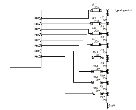
Figure 1 - Sine wave generation circuit diagram
How the circuit and program work
The circuit is basically a traditional R-2R ladder network use to generate analog sine wave output. If the proper type of resistor is used, the error at the output can be minimized.
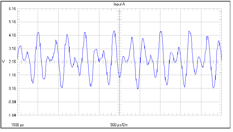
The program works by basically using a look up table to find the value of two sine waves and add them together to generate an instantaneous value for DTMF (dual tone multiple frequency) output. This value is then output to port B, which is weighted by the resistor values and generate a corresponding analog value. From the oscilloscope captured waveform shown below, we can see that the program is performing pretty well. The demo program uses the internal RC frequency of 4MHz. If an external 3.57945 MHz crystal is used, we can expect the output to be able to meet some telecom standards with minor tweaking.

The program starts by setting all port B pins to output and then generating tones corresponding to keys on a telephone keypad, i.e., 0-9, *, and #, by calling a dtmf generation routine called senddtmf.
Each key generates two tones which are then superimposed together. The instantaneous value of first sine wave is looked up and stored in the variable NEXTVALUE. Then the instantaneous value of the second sine wave is looked up and added into NEXTVALUE. Then we divide NEXTVALUE by 2 and output it to port B. This process is repeated at a constant interval until the loop count is exhausted. In the process, if we go to the end of a sine wave table, which is indicated by 127, we will loop back to the beginning of that table and continue.
Modifications and further options
Table lookup for sinusoidal signal generation provide efficient use of micro-controller time and code space. Even though other methods exist (for example, Z-transform method of sine wave generation), table lookup is still the best method, judging from our experience.
To eliminate the R-2R ladder, the readers may consider using an external A/D converter or combining this program with the virtual peripheral A/D documented in other application notes.
Fast Fourier Transform
Every electrical engineer has been exposed once or twice in his school days the good old Fourier series, where every kind of waveform can be represented by a series of sine and cosine waves. Based on his theorem,
¥
X(w ) = ò x(t) e -jw t dt
-¥
we can see that the frequency domain representation, X(w), of the time domain signal, x(t), is just x(t) multiplied by e-jwt or its more familiar equivalent, cos wt - j sin wt, integrated over all time. This will extract all elements of the waveform that has elements common with the sine and cosine signals.
This transform can be applied to discrete signals when we sample the continuous signal x(t) every T seconds and obtain x(nT), which in most cases, we abbreviate it to x(n) by setting T=1. Then we get,
¥
X(w ) = S x(n) e -jw n
n=-¥
In reality, we cannot ever processing an infinite signal due to limitation in time and space. But we would process a finite length signal, which gives us the Discrete Fourier Transform (DFT):
N-1
X(k) = 1/N S x(n) e -j (2p nk/N)
n=0
As we can see, N complex multiplications and N-1 complex additions are needed for each frequency point k. Since there are N frequency points (or bins) to be computed, we need N2 complex multiplications and N(N-1) complex additions.
A faster implementation is obviously needed. This problem was solved by the Fast Fourier Transform algorithm developed by Cooley and Tukey. They cleverly decomposed the DFT problem into smaller and smaller sub-transforms. The result is an algorithm that needs only N log2(N) complex multiplications. This is a significant savings as N increases.
Due to the complexity of the derivation of FFT, we will leave that to the more advanced textbooks that the readers may have access to and concentrate instead to how it is implemented on the SX.
How the program works
This program performs FFT on 16 points of 16 bit complex data. Each data point is represented by the real data followed by the imaginary data. If more RAM is present, then more data points can be handled.
The program starts by clearing all memory location and then loading a test pattern into the memory starting from $90 using the gen_test macro. Then the radix 2 FFT routine (radix 2 means that the smallest transform is operated on 2 data points) is called. After FFT is done, the result needs to be unscramble by calling the unscramble routine.
start
clr fsr ; reset all ram banks
:loop setb fsr.4 ; only second half is addressable
clr ind ; clear
ijnz fsr,:loop ; all
; fsr=0 on entry
gen_test ; Generate Test Vector Data
call R2FFT ; Compute Fourier Transform
page Unscramble
call Unscramble ; bit reverse the scrambled data
The gen_test macro reads data from the test_data table, which contains only the real part of data. The imaginary part is considered zero and automatically filled in as such.
To aid understanding, the radix 2 FFT algorithm can be represented in the following C program, which corresponds approximately one-to-one to the assembly language program. In the assembly language implementation, we used table lookup for implementing the sine and cosine functions due to time and space considerations.
#include <stdio.h>
#include <math.h>
void main()
{int i,j,k,l,m;
float Xi,Yi,Xl,Yl,Xt,Yt,sine,cosine,angle;
int data[32];
int count1,count2,quartlen,TF_offset,TF_addr;
const Fftlen=16;
const power=4;
const Scale=1;
for (i=0;i<32;i+=16)
{data[i]=0x0;data[i+1]=0;
data[i+2]=0x2d40;data[i+3]=0;
data[i+4]=0x3fff;data[i+5]=0;
data[i+6]=0x2d40;data[i+7]=0;
data[i+8]=0x0;data[i+9]=0;
data[i+10]=0xffffd2c0;data[i+11]=0;
data[i+12]=0xffffc001;data[i+13]=0;
data[i+14]=0xffffd2c0;data[i+15]=0;
}
for (m=0;m<32;m++) printf("[%d]=%x\n",m,data[m]);
count2=Fftlen;
quartlen=Fftlen/4;
TF_offset=1;
for (k=power;k>0;k--)
{
count1=count2;
count2=count2/2;
TF_addr=0;
printf("\nkloop k=%d\tcount1=%d\tcount2=%d\n",k,count1,count2);
for (j=0;j<count2;j++)
{
printf("\njloop j=%d\t",j);
angle=(float)TF_addr/16.0*(3.14159*2.0);
printf("TF_addr=%d\tangle=%f\t",TF_addr,angle);
sine=sin(angle);
cosine=cos(angle);
printf("sin=%f\tcos=%f\n",sine,cosine);
TF_addr+=TF_offset;
for (i=j*2;i<2*Fftlen;i=i+count1*2)
{
l=count2*2+i;
printf("\ni=%d\tl=%d\t",i,l);
Xl=data[l];Yl=data[l+1];
Xi=data[i];Yi=data[i+1];
Xt=Xi-Xl;
Yt=Yi-Yl;
printf("Xt=%f\tYt=%f\t",Xt,Yt);
Xi=Xi+Xl;
Yi=Yi+Yl;
printf("Xi=%f\tYi=%f\n",Xi,Yi);
if (Scale)
{
Xi/=2;Yi/=2;Xt/=2;Yt/=2;
}
Yl=cosine*Yt-sine*Xt;
Xl=cosine*Xt+sine*Yt;
printf("cosine*Yt=%f\tsine*Xt=%f\tYl=cosine*Yt-sine*Xt=%f\n",cosine*Yt,sine*Xt,Yl);
printf("cosine*Xt=%f\tsine*Yt=%f\tXl=cosine*Xt+sine*Yt=%f\n",cosine*Xt,sine*Yt,Xl);
data[l]=Xl;
data[l+1]=Yl;
data[i]=Xi;
data[i+1]=Yi;
}
}
TF_offset=2*TF_offset;
for (m=0;m<32;m++) printf("[%d]=%x\n",m,data[m]);
}
}
Time domain Frequency domain
Each cross represents a FFT operation called butterfly, which is:
= {x(t)+j y(t)} *( cos w - j sin w )
= x(t) cos w -j x(t) sin w + j y(t) cos w + y(t) sin w
= { x(t) cos w + y(t) sin w } + j {y (t) cos w - x(t) sin w }
At the end of the operations, the data points will be replaced by the real and imaginary part of the corresponding frequency bin. As we can see, more frequency bins mean higher spectral resolution.
Some note is necessary for the sine/cosine functions. Since the cosine function can be considered just a phase shifted version of sine function, they are combined together as such in the lookup table.
After all the operations, we can see that the results are in a bit reversed (scrambled) order. We have used some features of SX to simplify this operation. From the following code segment, we can see how bit 3 to bit 0 are reversed. This is considered quite efficient.
Unscramble
clr VarIloop ; i=0..15
reverse
clr VarL
snb VarIloop.3
setb VarL.0
snb VarIloop.2
setb VarL.1
snb VarIloop.1
setb VarL.2
snb VarIloop.0
setb VarL.3
The unscrambled results then represents the corresponding frequency bins.
Results and summary
The whole routine (including FFT, unscramble and sine table) occupies 455 words of program space. It uses 44 bytes of RAM for the routine and 64 bytes for the 16 point complex data, each of 16 bit wide.
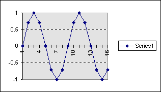
The test data is a piece of sine wave generated from the following table:
|
FFT * 16 |
FFT |
FFT |
FFT |
|||||
|
Point |
angle |
sin |
sin scaled |
sine scaled (hex) |
real part |
im part |
abs.mag. |
|
|
0 |
0 |
0 |
0 |
0000 |
0 |
0 |
0 |
0 |
|
1 |
0.785398 |
0.707107 |
11584.88 |
2D40 |
0 |
0 |
0 |
0 |
|
2 |
1.570796 |
1 |
16383.5 |
3FFF |
-1.30375548898498E-010-131068i |
-8.14847E-12 |
-8191.75 |
8191.75 |
|
3 |
2.356194 |
0.707107 |
11584.88 |
2D40 |
0 |
0 |
0 |
0 |
|
4 |
3.141593 |
1.23E-16 |
2.01E-12 |
0000 |
0 |
0 |
0 |
0 |
|
5 |
3.926991 |
-0.70711 |
-11584.9 |
FFFFFFD2C0 |
0 |
0 |
0 |
0 |
|
6 |
4.712389 |
-1 |
-16383.5 |
FFFFFFC001 |
0 |
0 |
0 |
0 |
|
7 |
5.497787 |
-0.70711 |
-11584.9 |
FFFFFFD2C0 |
0 |
0 |
0 |
0 |
|
8 |
6.283185 |
-2.5E-16 |
-4E-12 |
0000 |
0 |
0 |
0 |
0 |
|
9 |
7.068583 |
0.707107 |
11584.88 |
2D40 |
0 |
0 |
0 |
0 |
|
10 |
7.853982 |
1 |
16383.5 |
3FFF |
0 |
0 |
0 |
0 |
|
11 |
8.63938 |
0.707107 |
11584.88 |
2D40 |
0 |
0 |
0 |
0 |
|
12 |
9.424778 |
3.68E-16 |
6.02E-12 |
0000 |
0 |
0 |
0 |
0 |
|
13 |
10.21018 |
-0.70711 |
-11584.9 |
FFFFFFD2C0 |
0 |
0 |
0 |
0 |
|
14 |
10.99557 |
-1 |
-16383.5 |
FFFFFFC001 |
1.11431438295367E-010+131068i |
6.96446E-12 |
8191.75 |
8191.75 |
|
15 |
11.78097 |
-0.70711 |
-11584.9 |
FFFFFFD2C0 |
0 |
0 |
0 |
0 |
This corresponds to the following sine wave:

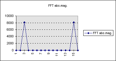
The result from FFT using the scaled sine data with Microsoft Excel is:

This is in accordance with the program output as seen in the following captured debug window. Here, Z(2) is FFFF+j E000 or (-1 +j -8192). Z(6) is j FFFF (j -1). And Z(14) is 0+ j 1FFE (0 + j 8190). The error is only minimal. To get the decimal equivalent, they must all be divided by 32767, which is the scaling factor.

Modifications and further options
To increase the number of data points, 8 bit data can be used so that 32 point FFT can be done. For further increase, we need to resort to the use of FFT for real data. This would demand a somehow significant modifications, which will allow us to process 64 point FFT.
With 8 bit data, the multiplication routine will become 8 x 8 and hence faster. This would increase the performance as well if 8 bit resolution of data is acceptable.
| file: /Techref/scenix/fft/fft.htm, 35KB, , updated: 1999/3/6 10:13, local time: 2025/10/4 19:10,
216.73.216.215,10-3-67-247:LOG IN
|
| ©2025 These pages are served without commercial sponsorship. (No popup ads, etc...).Bandwidth abuse increases hosting cost forcing sponsorship or shutdown. This server aggressively defends against automated copying for any reason including offline viewing, duplication, etc... Please respect this requirement and DO NOT RIP THIS SITE. Questions? <A HREF="http://techref.massmind.org/techref/scenix/fft/fft.htm"> </A> |
| Did you find what you needed? |
Welcome to massmind.org! |
|
The Backwoods Guide to Computer Lingo |
.